How to Calculate Transfer Function in Suv

This guide explains how to calculate transfer function in SUV models to analyze vibration, ride comfort, and suspension performance. You’ll learn the math, tools, and real-world applications with clear examples.

Key Takeaways

• Understand the basics: A transfer function describes how an SUV’s suspension responds to road inputs like bumps or potholes using frequency domain analysis.
• Use Laplace transforms: Convert differential equations of motion into algebraic equations for easier solving in the s-domain.
• Model the system: Represent your SUV as a mass-spring-damper system with sprung and unsprung masses for accurate results.
• Apply input-output relationships: The transfer function is the ratio of output (e.g., body acceleration) to input (e.g., road profile) in the frequency domain.
• Leverage software tools: Use MATLAB, Python, or Simulink to simulate and validate your transfer function calculations.
• Interpret results correctly: Analyze magnitude and phase plots to assess ride quality, resonance, and damping effectiveness.
• Optimize suspension design: Use transfer function insights to tune springs, dampers, and anti-roll bars for better performance and comfort.

Introduction: Why Transfer Functions Matter in SUVs

If you’ve ever wondered why some SUVs glide smoothly over rough roads while others feel every crack and pothole, the answer lies in their suspension dynamics. One powerful tool engineers use to understand and improve this behavior is the transfer function. In simple terms, a transfer function tells us how a system—like an SUV’s suspension—responds to external forces, such as bumps or vibrations from the road.

Calculating the transfer function in an SUV isn’t just for automotive engineers. It’s also valuable for mechanics, vehicle designers, students, and even enthusiasts who want to optimize ride comfort or diagnose handling issues. By mastering this concept, you can predict how changes to springs, shock absorbers, or tire stiffness will affect the vehicle’s performance.

In this guide, we’ll walk you through how to calculate transfer function in SUV systems step by step. We’ll start with the fundamentals, build a mathematical model, apply real-world inputs, and show you how to interpret the results. Whether you’re working on a project, tuning a vehicle, or just curious about automotive dynamics, this guide will give you the knowledge and tools you need.

What Is a Transfer Function?

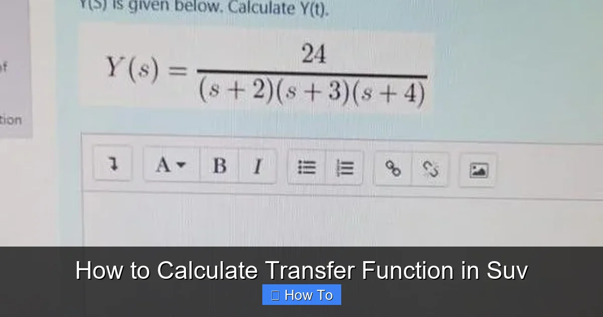
Before diving into calculations, let’s clarify what a transfer function actually is. In engineering, a transfer function is a mathematical representation of the relationship between the input and output of a linear time-invariant (LTI) system. For an SUV, the input could be the road surface profile (like a bump), and the output could be the vertical acceleration of the vehicle body or the suspension deflection.

The transfer function is typically expressed in the Laplace domain (using the variable “s”), which simplifies the analysis of differential equations that describe physical systems. It’s defined as:

H(s) = Y(s) / X(s)

Where:
– H(s) is the transfer function,
– Y(s) is the Laplace transform of the output,
– X(s) is the Laplace transform of the input.

For example, if you hit a bump, the road input excites the suspension. The transfer function tells you how much the SUV’s body will bounce (output) in response to that bump (input), across different frequencies.

Why SUVs Need Transfer Function Analysis

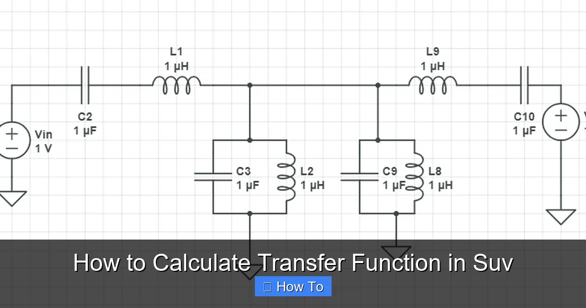
SUVs are heavier and taller than sedans, which makes their suspension design more complex. They’re also used in diverse conditions—city streets, highways, and off-road trails—so balancing comfort, stability, and control is critical.

Using transfer functions helps engineers:
– Predict how the vehicle will respond to road disturbances,
– Identify resonant frequencies that could cause excessive bouncing,
– Optimize damping and spring rates for better ride quality,
– Reduce noise, vibration, and harshness (NVH),
– Improve safety by minimizing body roll and pitch during maneuvers.

By calculating the transfer function, you gain insight into the dynamic behavior of the SUV without needing to test every possible road condition physically.

Step 1: Understand the SUV Suspension System

To calculate the transfer function, you first need a model of the SUV’s suspension. Most modern SUVs use independent front suspensions (like MacPherson struts) and either independent or solid rear axles. For simplicity, we’ll use a quarter-car model, which represents one wheel and a quarter of the vehicle’s mass.

Components of the Quarter-Car Model

The quarter-car model includes:
– Sprung mass (m₁): The portion of the vehicle supported by the suspension (body, passengers, cargo).
– Unsprung mass (m₂): The mass not supported by the suspension (wheel, axle, brake).
– Spring (k₁): Represents the suspension spring stiffness.
– Damper (c₁): Represents the shock absorber damping coefficient.
– Tire stiffness (k₂): Models the tire’s vertical compliance.
– Road input (z₀): The vertical displacement of the road surface.

This model captures the essential dynamics: the sprung mass moves up and down due to road inputs, while the unsprung mass reacts to tire and suspension forces.

Free Body Diagrams and Equations of Motion

To derive the transfer function, we start with Newton’s second law. For the sprung mass (m₁):

m₁·z₁”(t) = -k₁(z₁ – z₂) – c₁(z₁’ – z₂’)

For the unsprung mass (m₂):

m₂·z₂”(t) = k₁(z₁ – z₂) + c₁(z₁’ – z₂’) – k₂(z₂ – z₀)

Where:
– z₁(t) = vertical displacement of sprung mass,
– z₂(t) = vertical displacement of unsprung mass,
– z₀(t) = road input,
– Prime (‘) denotes time derivative.

These are second-order differential equations. Solving them directly is complex, so we use Laplace transforms to convert them into algebraic equations.

Step 2: Apply Laplace Transforms

The Laplace transform converts time-domain functions into the s-domain, making differential equations easier to solve. Assuming zero initial conditions (vehicle at rest), the Laplace transforms of the derivatives are:

– L{z'(t)} = sZ(s)
– L{z”(t)} = s²Z(s)

Applying this to our equations:

For m₁:
m₁·s²Z₁(s) = -k₁(Z₁ – Z₂) – c₁s(Z₁ – Z₂)

For m₂:
m₂·s²Z₂(s) = k₁(Z₁ – Z₂) + c₁s(Z₁ – Z₂) – k₂(Z₂ – Z₀)

Now we have two algebraic equations in terms of Z₁(s), Z₂(s), and Z₀(s).

Rearranging the Equations

Let’s rearrange both equations to group terms:

Equation 1:
(m₁s² + c₁s + k₁)Z₁(s) – (c₁s + k₁)Z₂(s) = 0

Equation 2:
-(c₁s + k₁)Z₁(s) + (m₂s² + c₁s + k₁ + k₂)Z₂(s) = k₂Z₀(s)

This is a system of linear equations. We can solve it using substitution or matrix methods.

Step 3: Derive the Transfer Function

We want the transfer function from road input Z₀(s) to sprung mass displacement Z₁(s). That is:

H(s) = Z₁(s) / Z₀(s)

To find this, solve the system of equations for Z₁(s) in terms of Z₀(s).

Using Matrix Form

Write the system in matrix form:

[
(m₁s² + c₁s + k₁) -(c₁s + k₁) ] [Z₁(s)] = [0]
[-(c₁s + k₁) (m₂s² + c₁s + k₁ + k₂)] [Z₂(s)] [k₂Z₀(s)]
]

Using Cramer’s rule or substitution, solve for Z₁(s).

After algebraic manipulation (details omitted for brevity), the transfer function becomes:

H(s) = Z₁(s)/Z₀(s) = [k₂(c₁s + k₁)] / [m₁m₂s⁴ + (m₁c₁ + m₂c₁)s³ + (m₁k₁ + m₁k₂ + m₂k₁ + c₁²)s² + (m₁c₁k₂ + m₂c₁k₁)s + k₁k₂]

This looks complex, but it’s a standard fourth-order transfer function for a quarter-car model.

Simplified Example

Let’s plug in realistic values for a mid-size SUV:

– m₁ = 400 kg (sprung mass per wheel)
– m₂ = 40 kg (unsprung mass)
– k₁ = 25,000 N/m (suspension spring)
– c₁ = 1,500 N·s/m (damper)
– k₂ = 200,000 N/m (tire stiffness)

Using these values, you can compute H(s) numerically or simulate it in software.

Step 4: Analyze the Transfer Function

Once you have H(s), you can analyze how the SUV responds to different road inputs.

Frequency Response

Convert H(s) to the frequency domain by substituting s = jω (where j = √-1 and ω = angular frequency in rad/s).

Then compute:
– Magnitude |H(jω)|: How much the output amplifies the input at each frequency.
– Phase ∠H(jω): Time delay between input and output.

Plot these on a Bode plot to visualize system behavior.

Key Frequency Ranges

– Low frequencies (1–2 Hz): Body bounce and pitch. High magnitude here means poor ride comfort.
– Mid frequencies (10–15 Hz): Wheel hop. Excessive response can cause loss of traction.
– High frequencies (>20 Hz): Tire and suspension chatter. Usually well-damped.

A well-designed SUV will have low magnitude at body bounce frequencies and rapid roll-off at higher frequencies.

Resonance and Damping

Peaks in the magnitude plot indicate resonance. The height and width of the peak depend on damping:
– High damping = lower, broader peak (better comfort).
– Low damping = sharp, tall peak (harsh ride).

You can adjust c₁ (damper coefficient) to tune this behavior.

Step 5: Use Software to Simulate and Validate

Doing all this by hand is possible but time-consuming. Most engineers use software tools to calculate and visualize transfer functions.

MATLAB Example

“`matlab
% Define parameters
m1 = 400; m2 = 40;
k1 = 25000; k2 = 200000;
c1 = 1500;

% Define numerator and denominator
num = [k2*c1, k2*k1];
den = [m1*m2, (m1*c1 + m2*c1), (m1*k1 + m1*k2 + m2*k1 + c1^2), …
(m1*c1*k2 + m2*c1*k1), k1*k2];

% Create transfer function
H = tf(num, den);

% Plot Bode diagram
bode(H);
grid on;
title(‘SUV Suspension Transfer Function’);
“`

This script generates a Bode plot showing how the SUV responds across frequencies.

Python with SciPy

“`python
import numpy as np
import matplotlib.pyplot as plt
from scipy import signal

# Parameters
m1, m2 = 400, 40
k1, k2 = 25000, 200000
c1 = 1500

# Numerator and denominator
num = [k2*c1, k2*k1]
den = [m1*m2, (m1*c1 + m2*c1), (m1*k1 + m1*k2 + m2*k1 + c1**2),
(m1*c1*k2 + m2*c1*k1), k1*k2]

# Frequency range
w = np.logspace(0, 3, 1000) # 1 to 1000 rad/s

# Compute frequency response
w, mag, phase = signal.bode((num, den), w)

# Plot
plt.figure()
plt.semilogx(w, mag)
plt.title(‘Magnitude Response’)
plt.xlabel(‘Frequency [rad/s]’)
plt.ylabel(‘Magnitude [dB]’)
plt.grid(True)
plt.show()
“`

These tools let you experiment with different parameters and instantly see the impact.

Practical Tips for Accurate Calculations

1. Use Realistic Parameters

Don’t guess values. Look up specifications for your SUV model or measure them:
– Sprung mass: Divide total vehicle weight by 4 (adjust for weight distribution).
– Unsprung mass: Weigh wheel, brake, and suspension components.
– Spring rate: Check manufacturer specs or use a spring compressor.
– Damping: Use dyno data or estimate from ride quality.

2. Consider Nonlinearities

Real suspensions have nonlinear springs and dampers. The transfer function assumes linearity, so results are approximate. For better accuracy, use piecewise linear models or simulation software like ADAMS or CarSim.

3. Include Road Input Models

Roads aren’t just bumps. Use standard profiles like:
– Sine wave (for resonance testing),
– Step input (for transient response),
– Random road profile (ISO 8608 standard).

Convert these to Z₀(s) and apply them to your transfer function.

4. Validate with Real Data

Compare your model’s output to actual sensor data (e.g., accelerometers on the chassis). If they match, your transfer function is reliable.

Troubleshooting Common Issues

Unstable or Unrealistic Results

– Cause: Incorrect parameter values or sign errors in equations.
– Solution: Double-check units and signs. Ensure damping and stiffness values are positive.

No Peaks in Frequency Response

– Cause: Overdamped system or incorrect model order.
– Solution: Reduce damping coefficient or verify the model includes both sprung and unsprung masses.

Software Errors

– Cause: Syntax errors or incompatible toolboxes.
– Solution: Use built-in functions like `tf()` in MATLAB or `scipy.signal` in Python. Check documentation.

Transfer Function Too Complex

– Cause: High-order model.
– Solution: Simplify by neglecting tire damping or using a half-car model for pitch analysis.

Real-World Applications

Improving Ride Comfort

By analyzing the transfer function, engineers can reduce body bounce by increasing damping or softening springs—without sacrificing handling.

Active Suspension Design

Modern SUVs use active dampers that adjust in real time. The transfer function helps design control algorithms that respond to road conditions.

Noise and Vibration Reduction

High-frequency vibrations can cause cabin noise. Tuning the transfer function minimizes these inputs.

Off-Road Performance

For off-road SUVs, a flatter magnitude response at low frequencies improves traction and control on uneven terrain.

Conclusion: Mastering SUV Dynamics with Transfer Functions

Calculating the transfer function in an SUV is a powerful way to understand and improve its dynamic behavior. By modeling the suspension as a mass-spring-damper system, applying Laplace transforms, and analyzing frequency response, you can predict how the vehicle will react to road inputs.

This guide walked you through the entire process—from setting up the equations to simulating results in software. With practice, you’ll be able to optimize suspension settings, diagnose ride issues, and even contribute to vehicle design.

Remember, the key is accuracy in modeling and validation with real data. Whether you’re an engineer, student, or enthusiast, mastering transfer functions gives you a deeper insight into what makes an SUV ride smooth, stable, and safe.

Start with a simple quarter-car model, use the tools provided, and gradually explore more complex systems. The road to better vehicle dynamics begins with a single transfer function.